Structured Prediction using Conditional Random Fields

In this tutorial, I would be explaining the concept of structured learning/prediction and the use of Conditional Random Fields (CRF) for achieving this. Before we start discussing about CRF’s, its essential that we understand what structure prediction is and why do we require it.

What is Structured Learning?

At present, Neural networks and its numerous variants are being applied for numerous fields from natural language processing to image classification. At its core, a Neural network takes a sample, along with its features, and propagates it through a set of weights (represented as layers) before finally making a prediction. Essentially it only considers one sample at time while making predictions. So at times, it could miss the big picture. If these samples are a part of a bigger element (image,sentence etc), it then doesn’t take into account the structure of the bigger element.

This is where structured prediction comes in. For problems like tokenizing a sentence or pixel be pixel classification of an image, its useful for the model to be aware of the overall structure of the sentence/image.

Lets take for example a pixel-by-pixel image classification problem consisting of human faces and the 6 output classes are

• eyes
• mouth
• nose
• hair
• skin (face region that doesnt include the other 4 classes)
• background

Now given a pixel to classify, we take into account its position in the overall image as well as the labels predicted for its neighbors. Suppose the given pixel is located exactly in the centre of the image, its more likely to be a nose pixel than a background pixel. On the other hand, if the pixel is at one of the corners of the image, then it is highly likely to be a background pixel than any other.

You also utilize the labels predicted for the neighborhood pixels. If the pixels right underneath the given pixel have been classified as nose pixels, then it is unlikely that the current pixel could be a mouth pixel. Similarly, if the pixels right above are classified as hair pixels, then it is unlikely that the given pixel is a background pixel.

This toy example should give you an idea as to what structured learning tries to achieve. In this case, we try to make our model learn the inherent structure of a human face. This concept can be applied to any problem in which the predictions have an inherent structure

---

 

Conditional Random Fields

Conditional Random Fields is one of the many algorithms that are used for structured prediction problems. CRF’s are the discriminative version of Hidden Markov Models (HMM). They are to HMM, what Logistic regression is to Naive Bayes. To get a better understanding of Discriminative vs Generative algorithms, check out these link1, link2

CRF is an  probabilistic graphical model. Essentially, you can imagine the CRF as a graph, with its set of vertices and edges and weights attached to each node as well as each edge. A CRF will have 2 types of weights , also known as potentials :

• Unary potentials – Given a particular node and its features, the unary potentials define how likely it is for the node to belong to a particular class
• Pair-wise potentials – Given that a neighboring node has been classified as a particular class, how likely is it for the current node to be classified as particular class.

You might find different formulation/symbols for CRF’s online, but at its core the CRF model consists of vertices, edges and potentials (Unary / Pair-wise).

 

 

The above figure depicts a Linear Chain CRF. As the name suggests, the structure of the output that we are gonna predict is linear in nature. This form of CRF is extensively used in Natural Language processing for Part-of-Speech tagging (POST). In the figure, X represents elements of the structured input (individual words in case of POST ) and Y represents the labels for each input (selected tags in case of POST). From the graph, we can see that the label Y_i depends on X_i as well as the labels predicted for Y_i-1 and  Y_i+1. 

---

 

PyStruct

PyStruct is one of the many open source CRF libraries found online. Compared to other libraries, PyStruct covers a variety of CRF variants and has better documentation. We will go though a very simple CRF example to understand how CRF training works. The example is on OCR Letter Sequence Recognition .

The dataset consists of written characters which are part of individual words. So a single training sample consists of all the characters of a word, except the first character. Now the first character has been removed from all words in order to avoid the effect of capital letters as they have a significantly different structure from the lowercase alphabets. Each character is an image of size 16×8.

import numpy as np
import matplotlib.pyplot as plt
import matplotlib.cm as cm

from sklearn.svm import LinearSVC

from pystruct.datasets import load_letters
from pystruct.models import ChainCRF
from pystruct.learners import FrankWolfeSSVM

def plotSample(x):
    n = len(x)
    plt.figure(1)
    for i in range(n):
        plt.subplot(100+n*10+i+1)
        plt.imshow(np.reshape(x[i],(16,8)) , cmap = cm.Greys)

letters = load_letters()
X, y, folds = letters['data'], letters['labels'], letters['folds']
X, y = np.array(X), np.array(y)
X_train, X_test = X[folds == 1], X[folds != 1]
y_train, y_test = y[folds == 1], y[folds != 1]

Use the plotSample function to take a look at some of the samples
plotSample(X_train[3])

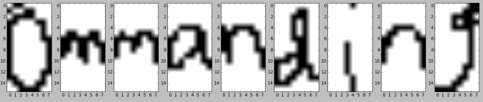
plotSample(X_train[16])

The above two samples are most likely from the words “commanding” and “embraces”.

---

 

We begin by defining the model that we shall use, which in this case is a Linear Chain CRF. The model defines the structure of the CRF in terms of how many states do each node have, what all edges are present in the model, which nodes are connected by an edge in the model etc. In short, it defines the overall structure and properties of the CRF “graph”.

Once the model is defined, we define the learner. Without going too much into the details, the learner is an algorithm that learns the unary/pairwise potentials based on the training data.

Another key component of a CRF model is the inference method. The inference method is the algorithm that finds the best solution given the sample and the potentials. This is an important parameter as depending on the problem that you are working on, one has to select the inference method suitably.

To understand the need for an inference algorithm, lets take the example of the above sample (X_train[16]). In most machine learning models, each of these characters are predicted individually.  So the first image “m” is evaluated and the most probable of the 26 alphabets is alloted. This is done for all the remaining 6 characters. This is equivalent to computing P(y_i|x_i). However, in CRF’s, we make predictions for all the characters of a sample in one go i.e P(Y|X), where Y = {y₁,y₂,y₃…y₇} and X = {x₁,x₂,x₃…x₇}. Therefore for this particular case, we have 26⁷ possibilities. As the number of possible solutions is huge, we need to have efficient algorithms to converge on the optimal solution.

Therefore , we could say that the 3 components of any CRF model are :

• Model
• Learner
• Inference method

model = ChainCRF()
ssvm = FrankWolfeSSVM(model=model, C=.1, max_iter=11)
ssvm.fit(X_train, y_train)

print("Test score with chain CRF: %f" % ssvm.score(X_test, y_test))

---

Now lets see the weights that the model has learned

ssvm.w
len(ssvm.w)

We see that there are 4004 elements in the weights vector. Lets see how we get to that. We know that there are 26 classes/states (corresponding to the 26 alphabets) in the CRF model.
Unary potenials
Each training sample is an array of length 128 (16×8). Therefore, in order to calculate the unary potential of a particular alphabet(class), we multiply the weights for the particular alphabet(class) with the training sample to derive the unary potential for that alphabet at that position. This weight vector is an array of length 128. Similarly, each alphabet(class) has its own set of weights. Therefore, all together, we have 3328 (26×128) weights to help define the unary potentials for all the classes.

Pairwise potentials
In this particular case , the edges of the CRF are directed as the probability of x after y is not the same as y after x. So is the probability of g after h when compared to h after g. Therefore considering all the pair-wise interactions, we have 676 (26×26) weights.

Therefore altogether, we have 4004 weights. The 3328 unary potentials are placed first in the ssvm.w vector after which the 676 pairwise potentials are placed.

---

 

The following plot given in the example gives a good visualization of the pairwise potentials.

abc = "abcdefghijklmnopqrstuvwxyz"
plt.matshow(ssvm.w[26 * 8 * 16:].reshape(26, 26))
plt.colorbar()
plt.title("Transition parameters of the chain CRF.")
plt.xticks(np.arange(25), abc)
plt.yticks(np.arange(25), abc)
plt.show()

From the above visualization, what we can understand is that the model has learned that after an “i”, “n” is very likely. Similarly, after a “l”, “y” is very likely. That seems accurate considering we just used  “similarly” and “likely” in the previous sentence.

Will be releasing another tutorial on training CRF’s using PyStruct soon!

Based on PyStruct , written by Andreas C. Mueller and Sven Behnke